All posts by Abhijit Joshi

Finding Nail Pops

I was trying to find a way to find nail pops in walls without hurting my eyes. The idea is to locate the nail pop and then put a bit of blue tape on it to mark its location for someone else who comes and fixes these things. And it suddenly came to me. Here we go. You will need the following:

  • a flashlight
  • a chair or ladder
  • blue tape (painters tape) and a pair of scissors
  • dark conditions (night-time is best)
  • a helper who can hold the flashlight (3 year old toddlers are ok!)

All you need to do is turn off all the lights and place the flashlight almost parallel to the wall. Sweep the entire wall with the beam of light and anything popping out by even a fraction of a millimeter will stand out as clear as day. 

Once you locate a pop, ask the flashlight holder to freeze and do your thing with the blue tape and scissors, using the chair and/or ladder if necessary. Continue sweeping all walls until done.

I’ll admit this is bit hard to do for ceilings, but it works in theory.


Tools for building a new website

My motivation for building a website was simple. I wanted to collect and organize important things from the last several years in one place for future reference. Something like an online portfolio of what I have been up to. Last I dabbled in HTML to create a website, I was a student at Clemson and was able to use my university servers for hosting my website. Apart from photos and other things, I remember my website had a dedicated section devoted to Tolkien’s Silmarillion. I also used the website for managing the classes I taught at Clemson, posting homework, test solutions and things of that sort.

Has a lot changed in 10 years? Looks like HTML5 is the latest and greatest, along with CSS3. As I am slowly discovering for myself, this adds several great features to help design good web pages. A book I particularly liked and have been using as a guide is HTML and CSS: Design and Build Websites by Jon Duckett.

One of the new HTML5 feature I’ve been using quite a lot is the <video> tag. Makes adding videos amazingly easy. I’m currently making movies using QuickTime (.MOV) and then converting them to .MP4 using Miro video converter. All my videos now play fine on Chrome and Safari. Need further testing to add support, if required, for Firefox and iOS devices.

Another useful feature I absolutely wanted was syntax highlighting for C/C++ code. One way to get this feature on your webpage is via prism (http://prismjs.com/). This essentially supplies a .css file and a JavaScript file that you link to in your HTML file. Once you do this, simply wrap your code within <pre><code class=”lang-cpp”> and </code></pre>.

Finally, the question of where to host the site. I decided to go with iPage and it’s been a great experience so far.  So to summarize all the things needed to build a new website from scratch:

  • iPage
  • A good reference book for HTML and CSS
  • QuickTime for recording video from the screen
  • Miro video converter
  • Prism for syntax highlighting of C/C++ code
  • Lots of time and patience


2D Heat Conduction – Solving Laplace’s Equation on the CPU and the GPU

Laplace’s equation is one of the simplest possible partial differential equations to solve numerically. It applies to various physical processes like electric potentials and temperature fields. In this blog, I will highlight a simple numerical scheme to solve this equation referred to as Jacobi iteration. Starting with a simple CPU based C++ code, I will highlight how easy it is to port this code to the GPU using CUDA.

We’ll focus on a particular example from heat transfer, where the goal is to solve for the steady-state temperature field T(x,y) and the solution domain is a square of size L in the X-Y plane. The boundary conditions are as follows:

  • Left edge: x = 0, T(0, y) = 1
  • Right edge: x = L, T(L, y) = 0
  • Bottom edge: y = 0, T(x,0) = 0
  • Top edge: y = L, T(x,L) = 0

Without going into too many details, the core algorithm for solving the temperature field inside the domain boils down to this simple equation:

T(i,j) = 0.25 * [T(i-1,j) + T(i+1,j) + T(i,j-1) + T(i,j+1)]       ——-   (1)

Here, it is assumed that the square domain is represented using a computational grid of N x N points, equally spaced along X and Y. Equation (1) essentially states that the temperature value at any node point equals the arithmetic average of the 4 neighboring temperature values. The value at the boundary node points are known from the boundary conditions and the objective is to iteratively find the interior T(i,j) values using Eq.(1).

The CPU approach

We define two 2D arrays, T(1:N,1:N) and T_new(1:N,1:N) and essentially loop over all interior node points in the domain, updating T_new(i,j) at each interior node point using values from T(i,j) from the previous iteration. The core Jacobi function from the CPU code is copied below for reference.

void Jacobi(float* T, float* T_new)
{
    const int MAX_ITER = 1000;
    int iter = 0;

    while(iter < MAX_ITER)
    {
        for(int i=1; i<NX-1; i++)
        {
            for(int j=1; j<NY-1; j++)
            {
                float T_E = T[(i+1) + NX*j];
                float T_W = T[(i-1) + NX*j];
                float T_N = T[i + NX*(j+1)];
                float T_S = T[i + NX*(j-1)];
                T_new[i+NX*j] = 0.25*(T_E + T_W + T_N + T_S);
            }
        }

        for(int i=1; i<NX-1; i++)
        {
            for(int j=1; j<NY-1; j++)
            {
                float T_E = T_new[(i+1) + NX*j];
                float T_W = T_new[(i-1) + NX*j];
                float T_N = T_new[i + NX*(j+1)];
                float T_S = T_new[i + NX*(j-1)];
                T[i+NX*j] = 0.25*(T_E + T_W + T_N + T_S);
            }
        }
        iter+=2;
    }
}

In this implementation, we update T_new(i,j) using values from T(i,j) and then update T(i,j) using values from T_new(i,j). This essentially completes two Jacobi iterations. We keep going until a set number of maximum iterations is reached (1,000 in the above code snippet). The CPU implementation is slow mainly because we update points in a sequential fashion, one after the other. But this was pretty much the best you could hope for before parallel computing.

The GPU approach: CUDA

Notice that each update of T_new(i,j) in the above code is independent of every other update. So what if we could update all node points in parallel at the same time? This is exactly what we do using GPUs.

Click here to download the GPU (CUDA) code

Notice that the basic instruction for updating the node point using the average of its neighbors is identical in the GPU code. However, the loop over i and j has disappeared in the kernel (function running on the GPU). The key point to understand is that this kernel is executed in parallel using several threads on the GPU using the triple chevron notation <<<   >>>.

Each thread figures out which node point it is updating and updates the value in the appropriate memory location. When all threads are done updating their node point, we move on to the next iteration. Obviously, the GPU approach is faster than the CPU approach, but there is also some time spent in allocating resources on the GPU and in copying data from the CPU to the GPU. Thus, the speed up in the actual execution of the Jacobi iteration may not become apparent until the mesh size is large.

RESULTS

In the figure below, a comparison of the run-time between the CPU and the GPU is attached. For the largest grid shown below, we obtained a speed up of 143X for the CUDA version compared to the CPU code.

laplaceCUDA

It will be apparent that the GPU version using CUDA is way faster than the CPU version for mesh sizes larger than 256 x 256. In reality, as mentioned above, the actual Jacobi iteration (or convolution) part is always faster than the CPU version.

To conclude, this example illustrated how a simple partial differential equation (PDE) can be solved on the GPU provided we can execute it as a “single instruction on multiple data” (SIMD) algorithm. The basic idea of creating a workspace (array) on the GPU and updating elements of this array in parallel can be applied even to more complex PDEs and algorithms, provided they can be written in a SIMD fashion. The only limitation in this approach is the amount of memory available on the GPU.

Lattice Boltzmann Method: Moving from CPU to GPU

Over the last couple of decades, the lattice Boltzmann method (LBM) has grown into a potent alternative methodology for computational fluid dynamics (CFD). As such, CFD has been traditionally developed using the Navier-Stokes equations as a starting point. But there are several advantages to using the LBM, chiefly the extreme simplicity of the approach (easy coding) and the inherently parallel nature of the computations (scales easily to large machines). The LBM is akin to an explicit numerical scheme, in that the variable at the new time level can be calculated based on the (local) values of the variable at the previous time level.

Unlike regular CFD, where the primary dependent variables are the velocity components, the density and the pressure, the LBM works with particle velocity distribution functions, or PDFs. A simplified way of understanding the LBM is to imagine that there are a set of discrete points in space (lattice points) and there is a set of finite directions at each lattice point along which fluid particles can move or “stream”. During each time step, particles “stream” or hop from one lattice point to another along these finite directions and then “collide” with each other, conserving mass and momentum. This collision event leads to a new distribution of particles, which then streams again to neighboring lattice points. For more information about the LBM, you can refer to several excellent review articles available on the internet.

A simple application of the LBM is to solve for two-dimensional flow inside a square cavity. In this problem, the square cavity is completely filled with a constant viscosity fluid. The three side walls of the cavity are fixed and the top wall suddenly starts moving to the right with a constant velocity, dragging the adjacent fluid along with it and causing a re-circulating flow to develop inside the cavity. In this blog, we will provide a canonical LBM implementation of this problem (for low Reynolds numbers) and provide detailed CPU and GPU versions of the code so interested users can see for themselves how easy it is to migrate from the C++ (CPU version)  to the CUDA (GPU version) and the amazing speed-up than can result from doing so.

The CPU approach

A simple LBM code that can be implemented on the CPU can be obtained by following the link below. This 2D implementation uses the D2Q9 model, which means we have a 2 dimensional model with 9 discrete velocity directions.

Click here to download the CPU code

The CPU version sweeps through each lattice point in a sequential manner and finds the new distribution functions after streaming and collision at that lattice point. However, all of these updates are completely independent of each other and they can be performed in parallel.

The GPU approach

The basic idea behind this particular GPU implementation is very simple. We allocate and initialize all the relevant arrays directly on the GPU. Once this is done (we will assume that we have enough memory to accomplish this task), the actual updating of the PDFs because of streaming and collision is performed in parallel using thousands of threads that each work on independent lattice points. The complete CUDA code for implementing this idea is provided below for reference. As we said, this is just a demonstration of how to port the CPU based C++ code to the GPU and we do not wish to imply that this is the best and most efficient implementation of the LBM on the GPU. But a code is worth a thousand words:

Click here to download the GPU code

The initial part of the code starts off on the CPU and allocates space to store the PDF arrays on the GPU using cudaMalloc. After this, the main portion of the algorithm runs completely on the GPU. The only instance where we would be required to move data from the GPU to the CPU is when we want to write it to output files for post-processing purposes. This is not done in this example for clarity and conciseness.

RESULTS

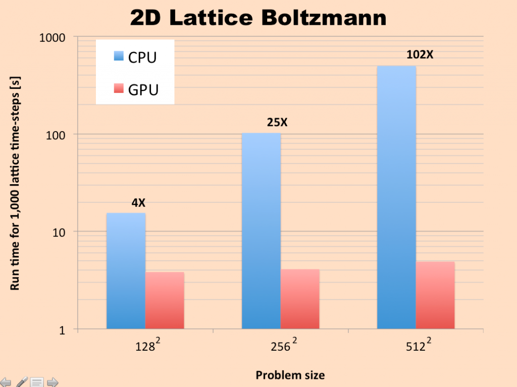
We ran this problem using both the CPU version and the GPU version for a range of grid sizes, starting from a 128 x 128 lattice and going up to a 512 x 512 lattice. The results for total simulation time are summarized in the graph below. It can be observed that the GPU version completely outperforms the CPU version, even for the 128 x 128 grid.

Screen Shot 2013-03-25 at 2.11.49 PM